Naive Bayes classifier – a naive introduction (with R)

[Supervised (non-linear) classification method]

Naive Bayes is a probabilistic classifier based on i) Bayes’ theorem and ii) a strong (“Naive”) assumption on the independence of all \(p\) features (variables) within each class.

Naive Bayes: the gist of it

• resource efficient & fast
• scales well
• works well when the number of samples \(n\) is small relative to the number of features \(p\)

From Bayes’ theorem, our objective is to estimate the posterior (conditional) probability for an observation of belonging to class k given its predictor variables: \(P(Y=k | X)\). A bit of nomenclature:

• observations: our records (e.g. individual subjects)
• class k: the class to which each observation belongs (e.g. case/control)
• (predictor) variables: “things” that have been measured on our observations (e.g. blood parameters)
• prior: initial probability of belonging to class k

posterior = (prior * likelihood) / evidence

We therefore need:

• estimates of the priors \(p_k\) for each class (e.g. relative frequencies of the k classes in the training data)
• estimates of the likelihood \(f_k(x)\) (probability of the data for each class k)
• evidence: sum of the probability of the data (likelihood) over all classes (total probability of the data)

Under the naive assumption of independence of the predictor variables within classes, we non longer need to calculate complex joint probability distributions of the p variables, and the likelihood of the data for each class is given by the product of the densities of each of the p predictors in that class:

\[f_k(x) = f_{k1}(x_1) \cdot f_{k2}(x_2) \cdot\ldots f_{kp}(x_p)\]

Mind you that these are the densities for individual variables in each class, i.e. the sub-components of the likelihood (and of the evidence when summed over the k classes). These sub-components (predictor variable densities per class) are the key ingredients of the Naive Bayes classifier, and can be estimated in a number of ways:

• from univariate normal distributions: \(x_p\|k\) \(\sim N(mean(x_{pk}),var(x_{pk}))\)
• non parametrically, as the fraction of the training observations in the \(k_{th}\) class that belong to the same histogram bin for the different values (ranges) of \(x_p\)
• using a kernel density estimator (a smoothed version of the above histogram)
• if \(x_p\) is qualitative, from the relative frequencies of observations in class k having the different values of \(x_p\) (e.g. proportions of males and females in the class)

The assumption of Naive Bayes is clearly far from true, but provides a good approximation, especially when n is not large enough relative to p to provide effective estimates of \(f_k(x)\).

By simplifying the problem, Naive Bayes introduces some bias but reduces the variance of the classifier. We expect to see a great pay-off to using naive Bayes in instances where p is large or n is small, so that reducing the variance is very important (the bias-variance trade-off).

Further (important) details

1. the data can be transformed (e.g. normalized) and an estimator may need to be chosen (Gaussian, histogram frequency, kernel density, class frequency for categorical variables etc.): transformations of the data and selection of the estimator(s) are part of the modelling and fine-tuning process.
2. Caveat: when \(P(x_p | y=k) = 0\) (a specific value of the \(x_p\) predictor never occurs in class k), the overall likelihood of the data under the Naive Bayes assumption would go to zero (product of all $x_p$) \(\rightarrow\) the Laplace smoother: adds a small number to the frequencies for each feature (variable, predictor) in class k (how much? \(\rightarrow\) again, a tuning hyperparameter!)

An example in R

There are many R packages that implement the Naive Bayes classifier in R: e.g. e1071, klaR, naivebayes, bnclassify, caret, h2o

Here we look at an illustration using the caret + klaR packages (caret is a wrapper for many other R packages that provide a unified framework for statistical/machine learning).

As example, data on the root vigor (yes/no) and SNP genotypes of sugar beet (Beta vulgaris) are used. The dataset comes from Biscarini et al. 2016, and contains \(15\%\) swapped labels (classes).

The datasets is a data.frame with n samples (rows) and m columns (the predictor variables – SNP genotypes coded as 0/1/2 in tyhis case). One additional column is the class (label): in this case, 0/1 for presence/absence of root vigor. Initially, we read the data (data.table::fread()) then change the label to a factor (to avoid it being confused as a numeric value), and convert the data to a tibble (details here) [if you want, you can try the code below with the Iris flower dataset: in R, data(iris): Species is the target class to predict based on four sepal and petal variables]

rootv = mutate(rootv, classe = as.factor(classe)) %>% 
	as_tibble()

First, a little preprocessing:

## remove predictors with zero variance
nzv0 = nearZeroVar(rootv[rootv$classe=="0",], saveMetrics = TRUE)
nzv1 = nearZeroVar(rootv[rootv$classe=="1",], saveMetrics = TRUE)
 
nzv = (nzv0$nzv | nzv1$nzv)
nzv[length(nzv)] <- FALSE ## this is the target label, obviously with zero variance within class (restored to FALSE to be kept in the data)-nzv
 
rootv = rootv[, !(nzv)]

Then, we set up the model: split in training and test data partitions, specify the cross-validation setting and the grid value for the hyperparameters to tune.

## 1) data split
split <- initial_split(rootv, prop = .8, strata = "classe")
train <- training(split)
test  <- testing(split)
 
## 2) create response and feature data
features <- setdiff(names(train), "classe")
x <- train[, features]
y <- train$classe
 
## 3) set up 5-fold cross validation procedure
train_control <- trainControl(
  method = "cv", 
  number = 5
  )
 
## 4) set up tuning grid
search_grid <- expand.grid(
  usekernel = c(TRUE, FALSE),
  fL = 0:3,
  adjust = seq(1, 5, by = 1) ## bandwidth of the kernel density estimator (larger values --> more flexible estimator)
)

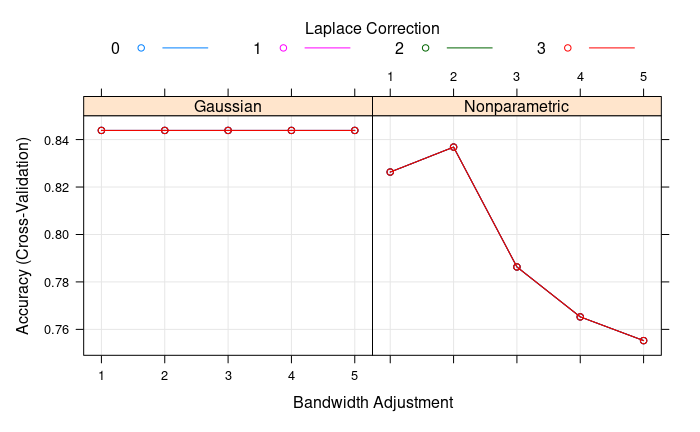
Now we can train the model: we see that we are better off with the Gaussian estimate of the predictor variable densities (the key ingredients of Naive Bayes!) and there’s no need of the Laplace smoother (no variables with zero density within class).

# train model
nb.m2 <- train(
  x = x,
  y = y,
  method = "nb",
  trControl = train_control,
  tuneGrid = search_grid
  )

Finally, we make predictions on the test set and we get a final accuracy of 0.76 (6 wrong predictions on the 25 test observations).

## making predictions on the test set
pred <- predict(nb.m2, newdata = test)
confusionMatrix(pred, test$classe)

home